QuantStudio Real-Time PCR software 是我们经常使用的 RT-PCR 软件, 它上面的可视化只能简单看看, 不满足发论文的需求. 如果需要得到发表级的图片, 还是需要 用 ggplot 大法加持.
为了能够使用这些数据, 首先需要导出文件. 为了方便操作, 文件导出时, 选择 *.txt 格式, 每个面板导出成一个单独文件. 将文件放在 data 文件夹中.
数据预处理
根据文件名后缀找到数据.
# 数据文件目录
dir <- "data"
options(stringsAsFactors = F)

# 根据文件名后缀找到对应文件
amplification_file <- list.files(path=dir,full.names = T,pattern = "Amplification Data_ViiA7_export.txt")
result_file <- list.files(path=dir,full.names = T,pattern = "Results_ViiA7_export.txt")
meltcurve_file <- list.files(path=dir,full.names = T,pattern = "MeltCurve Data_ViiA7_export.txt")
我们使用 readr 来读取数据. 这个包避免了 R 语言对列名不合时宜的转换.
每个文件的前面 43 列都是基本描述信息, 选择略过. 读取接下来的数据表格.
在 results 文件中, CT 值的缺失值用 "Undermined" 表示. 另外, 该文件末尾的也需要检查一下, 如果有非数据信息要删掉. 否则读取文件会报错.
# 读取文件
library(tidyr)
library(dplyr)
## Warning: 程辑包'dplyr'是用R版本4.0.5 来建造的##
## 载入程辑包:'dplyr'## The following objects are masked from 'package:stats':
##
## filter, lag## The following objects are masked from 'package:base':
##
## intersect, setdiff, setequal, unionlibrary(readr)
# read
amplification <- read_delim(amplification_file,"\t",skip = 43)##
## -- Column specification --------------------------------------------------------
## cols(
## Well = col_double(),
## Cycle = col_double(),
## `Target Name` = col_character(),
## Rn = col_double(),
## `Delta Rn` = col_double()
## )raw_results <- read_delim(result_file,"\t",skip = 43,na = "Undetermined")##
## -- Column specification --------------------------------------------------------
## cols(
## .default = col_logical(),
## Well = col_double(),
## `Well Position` = col_character(),
## `Sample Name` = col_character(),
## `Target Name` = col_character(),
## Task = col_character(),
## Reporter = col_character(),
## Quencher = col_character(),
## CT = col_double(),
## `Ct Mean` = col_double(),
## `Ct SD` = col_double(),
## `Ct Threshold` = col_double(),
## `Baseline Start` = col_double(),
## `Baseline End` = col_double(),
## Tm1 = col_double(),
## Tm2 = col_double(),
## Tm3 = col_double(),
## MTP = col_character(),
## EXPFAIL = col_character(),
## HIGHSD = col_character(),
## NOAMP = col_character()
## # ... with 1 more columns
## )
## i<U+00A0>Use `spec()` for the full column specifications.meltcurve <- read_delim(meltcurve_file,"\t",skip = 43)##
## -- Column specification --------------------------------------------------------
## cols(
## Well = col_double(),
## `Well Position` = col_character(),
## Reading = col_double(),
## Temperature = col_double(),
## Fluorescence = col_double(),
## Derivative = col_double()
## )在 "Results" 文件中, 含有我们定义的 "Sample Name" 和 "Target Name", 而在另外两个文件中不存在. 为了能够在图中显示这些信息, 我们需要将这些信息提取出来, 并添加到另外两个文件数据中. 添加时, 按照 "Well" 合并即可.
# 修整数据
meta <- raw_results %>% select(Well, `Sample Name`, `Target Name`)
amplification <- amplification %>% select(Well,Cycle,Rn,`Delta Rn`) %>%
  left_join(meta) %>%
  filter(Well<=5)
## Joining, by = "Well"meltcurve <- meltcurve %>%
select(Well,Reading,Temperature,Fluorescence,Derivative) %>%
filter(!is.na(Fluorescence)) %>%
left_join(meta)%>%
filter(Well<=5)## Joining, by = "Well"可视化
扩增曲线
首先绘制扩增曲线. 扩增曲线描述 RT-PCR 荧光信号随循环数的变化情况.
library(ggplot2)

# 更好看的科学计数法
fancy_scientific <- function(l) {
  # turn in to character string in scientific notation
  l <- format(l, scientific = TRUE)
  # quote the part before the exponent to keep all the digits
  l <- gsub("^(.*)e", "'\\1'e", l)
  # turn the 'e+' into plotmath format
  l <- gsub("e", "%*%10^", l)
  # remove +
  l <- gsub("\\+","",l)
  # return this as an expression
  parse(text=l)
}

ggplot(amplification,aes(Cycle,Rn,group=Well, color=`Target Name`,shape=`Sample Name`)) +
  geom_line() +
  scale_y_continuous(labels=fancy_scientific)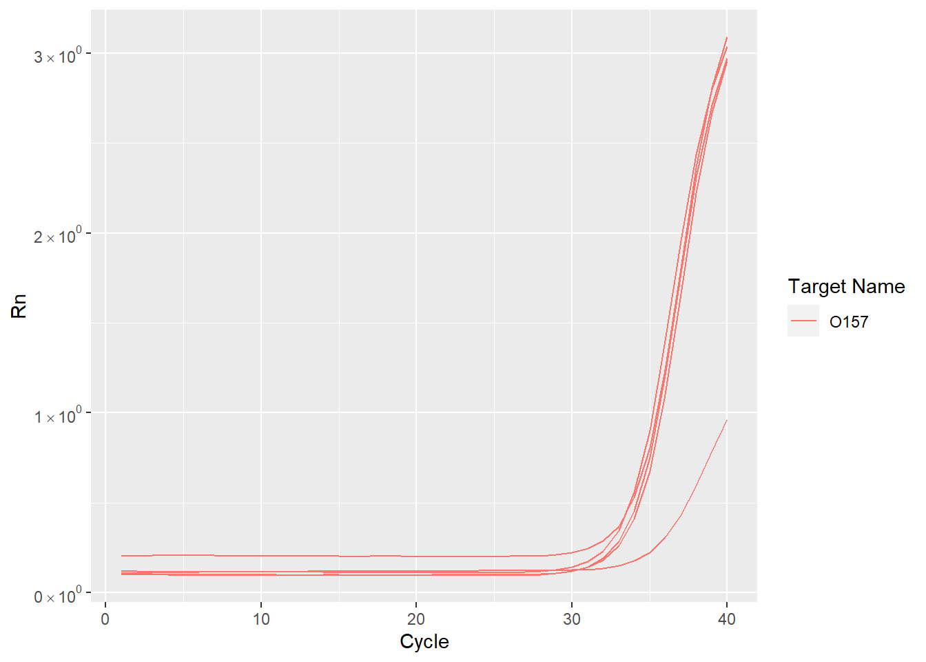
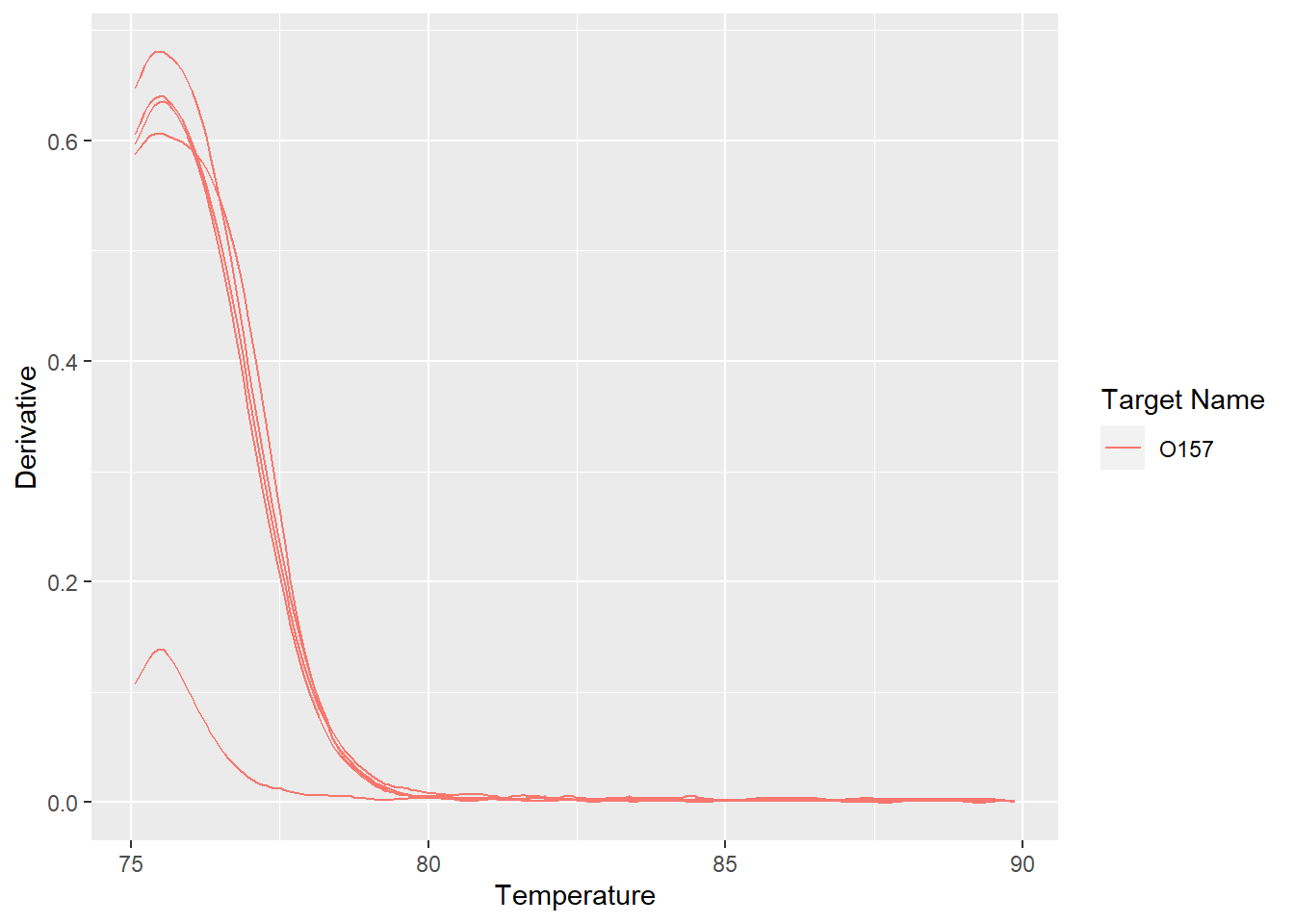
溶解曲线
溶解曲线可以看出扩增产物的特异性.
ggplot(meltcurve,aes(Temperature,Derivative,group=Well,color=`Target Name`)) +
  geom_line()